Convolution transform#

Wildboar implements two convolutional transformation methods Rocket [1] and Hydra [2], described by Dempsar et al. Both algorithms employ random convolutional kernels, but in sligtly different manners. In Rocket, each kernel is applied to each time series and the maximum activation value and the average number of positive activations are recorded. In Hydra, the kernels are partitioned into groups and for each exponential dilation and padding combination each kernel is applied to each time series and the number of times and the number of times each kernel has the highest activation value and the lowest is recorded. Then the features corresponds to the number of times a kernel had the in-group highest activation and the average of the lowest activation.

For the purpose of this example, we load the MoteStrain dataset for the UCR time series archive and split it into two parts: one for fitting the transformation and one for evaluating the predictive performance.

from wildboar.datasets import load_dataset
from sklearn.model_selection import train_test_split

X, y = load_dataset("MoteStrain")
X_train, X_test, y_train, y_test = train_test_split(X, y, random_state=1)

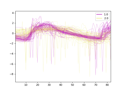
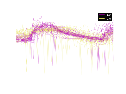
The dataset contains 954 samples with 84 time steps each. Of the samples, 510 is labeled as 1.0 and 444 labeled as 2.0. Here, we plot the time series.

Hydra transformation#

In Wildboar, we extensively utilize the functionalities of scikit-learn and can directly employ these features. We construct a pipeline wherein we initially transform each time series into the representation dictated by Hydra (utilizing the default parameters n_groups=64 and n_kernels=8). The subsequent stages of the pipeline include the application of a sparse scaler, which compensates for the sparsity induced by the transformation (it is important to note that we count the frequency of occurrences where a kernel exhibits the highest activation, and in numerous instances, a single kernel may never achieve this), and ultimately, the pipeline employs a standard Ridge classifier on the transformed data.

from wildboar.datasets.preprocess import SparseScaler
from wildboar.transform import HydraTransform

from sklearn.pipeline import make_pipeline

hydra = make_pipeline(HydraTransform(random_state=1), SparseScaler())
hydra.fit(X_train, y_train)

Pipeline(steps=[('hydratransform', HydraTransform(random_state=1)),
                ('sparsescaler', SparseScaler())])

In a Jupyter environment, please rerun this cell to show the HTML representation or trust the notebook.
On GitHub, the HTML representation is unable to render, please try loading this page with nbviewer.org.

We can inspect the resulting transformation by using the transform function.

X_test_transform = hydra.transform(X_test)
X_test_transform[0]

array([ 0.53921955, -0.39192971, -0.60035454, ..., -0.36929508,
        0.5286341 ,  1.08999765])

The transformed array contains 4096 features.

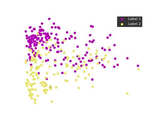
We can use principal component analysis (PCA) to identify the combination of attributes that account for most of the variance in the data.

Download plot source

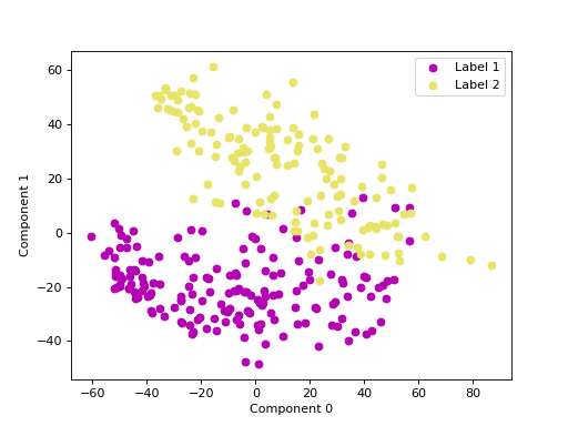
The first two components explain 23.04 and 17.10 percent of the variance.

Rocket transform#

The Rocket transformation employs a large, randomly generated set of kernels to enable the transformation process. By default, the parameter n_kernels is assigned the value of \(10000\) kernels. Furthermore, we utilize the pipelines offered by scikit-learn to normalize the feature representation, ensuring a mean of zero and a standard deviation of one.

from sklearn.preprocessing import StandardScaler

from wildboar.transform import RocketTransform

rocket = make_pipeline(RocketTransform(), StandardScaler())
rocket.fit(X_test, y_test)

Pipeline(steps=[('rockettransform', RocketTransform()),
                ('standardscaler', StandardScaler())])

In a Jupyter environment, please rerun this cell to show the HTML representation or trust the notebook.
On GitHub, the HTML representation is unable to render, please try loading this page with nbviewer.org.

We can inspect the resulting transformation.

X_test_transform = rocket.transform(X_test)
X_test_transform[0]

array([-0.80749201, -0.5376525 , -0.69224202, ..., -0.6422479 ,
       -0.21959721, -0.24136447])

In contrast to Hydra whose transformation size depends on the number of time steps in the input, the Rocket transformation has a fixed size only dependent on the number of kernels. As such, the resulting transformation consists of \(10000\) features.

We can use principal component analysis (PCA) to identify the combination of attributes that account for most of the variance in the data.

Download plot source

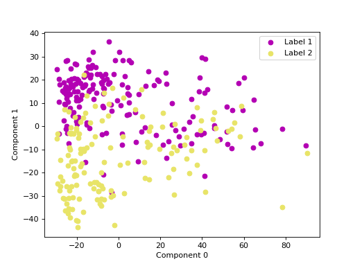
The first two components explain 35.06 and 17.45 percent of the variance.