Counterfactual explanations

Counterfactual explanations for time series classification provide changes that describe how a slightly different time series instance could have led to an alternative classification outcome. Essentially, they identify the minimum changes needed to alter the input time series, such as changing certain values at specific time points, in order to flip the model’s decision from one class to another. These explanations can help users understand model behavior and decision-making by highlighting critical points in time and the nature of the data that would need to be different for a different result.

Nearest neighbour counterfactuals

Wildboar facilitates the generation of counterfactual explanations for time series classified by k-nearest neighbors classifiers. Presently, two algorithms are implemented for this purpose. The initial algorithm, as delineated by Karlsson et al. [1], employs the arithmetic mean of the k-nearest time series belonging to the contrasting class. The alternative algorithm utilizes the medoid of the k-nearest time series. These algorithms are incorporated within the class KNeighborsCounterfactual. The parameter method is provided to select between the two counterfactual computation methods.

Although the approaches might appear similar, the former is applicable exclusively to KNeighborsClassifier configured with the metric parameter set to either dtw or euclidean, and to sklearn.neighbors.KNeighborsClassifier when the metric parameter is specified as euclidean or as minkowski with p=2. The latter approach is applicable to any metric configuration.

To generate counterfactuals, we first need to import the require classes. In this example we will be using KNeighborsClassifier and explain the classification outcome using KNeighborsCounterfactual. We also load load_dataset to download a benchmark dataset.

from wildboar.datasets import load_dataset
from sklearn.model_selection import train_test_split

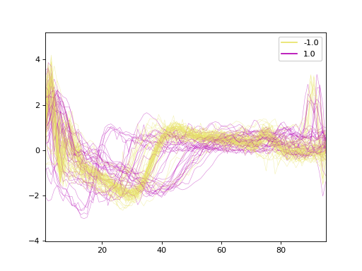
In this example, we will make use of the ECG200 dataset, which contains electrocardiogram (ECG) signals and is used for binary classification tasks. It contains time series data representing ECG recordings, where the goal is to distinguish between normal heartbeat signals and those that correspond to a particular type of abnormal cardiac condition. Each time series in the ECG200 dataset corresponds to an ECG signal, and the classes represent whether the signal is from a normal heart or one with a specific anomaly.

X, y = load_dataset("ECG200")
X_train, X_test, y_train, y_test = train_test_split(X, y, random_state=1)

The dataset contains 150 samples with 96 time steps each. Of the samples, 50 is labeled as -1.0 and 100 labeled as 1.0. Here, we plot the time series.

Next we fit a k-nearest neighbors classifier with five neighbors using Dynamic Time Warping.

from wildboar.distance import KNeighborsClassifier
nn = KNeighborsClassifier(n_neighbors=5, metric="dtw", metric_params={"r": 0.5})
nn.fit(X_train, y_train)

KNeighborsClassifier(metric='dtw', metric_params={'r': 0.5})

In a Jupyter environment, please rerun this cell to show the HTML representation or trust the notebook.
On GitHub, the HTML representation is unable to render, please try loading this page with nbviewer.org.

The resulting estimator has an accuracy of 84.0%.

To compute counterfactuals, we utilize the KNeighborsCounterfactual class from the counterfactual module. A counterfactual explainer comprises two primary methods for interaction: fit(estimator) and explain(X, desired_label). The fit method requires an estimator for which the counterfactuals are to be constructed, while the explain method requires an array of time series to be modified and an array of the desired labels. In the provided code example, we initially predict the labels for each sample in X and subsequently create a new array of desired labels to construct counterfactuals predicted as label -1 for all samples initially predicted as 1 and vice versa. Subsequently, we fit the counterfactual explainer to the estimator and calculate the counterfactuals. Since the method parameter is set to "auto", the explainer will utilize the k-means algorithm and assign the nearest cluster centroid at which the classifier is expected to predict the target class.

from wildboar.explain.counterfactual import KNeighborsCounterfactual
def find_counterfactuals(estimator, explainer, X):
   y_pred = estimator.predict(X)
   y_desired = np.empty_like(y_pred)

   # Store an array of the desired label for each sample.
   # We assume a binary classification task and the the desired
   # label is the inverse of the predicted label.
   a, b = estimator.classes_
   y_desired[y_pred == a] = b
   y_desired[y_pred == b] = a

   # Initialize the explainer, using the medoid approach.
   explainer.fit(estimator)

   # Explain each sample in X as the desired label in y_desired
   X_cf = explainer.explain(X, y_desired)
   return X_cf, y_pred, estimator.predict(X_cf)

explainer = KNeighborsCounterfactual(random_state=1, method="auto")
X_cf, y_pred, cf_pred = find_counterfactuals(nn, explainer, X_test)
X_cf

array([[0.7757554 , 1.04521294, 1.12209986, ..., 0.41066892, 0.51301643,
        0.13364922],
       [0.4545415 , 0.8152728 , 2.36613719, ..., 0.59799892, 0.6364614 ,
        0.66240546],
       [0.7757554 , 1.04521294, 1.12209986, ..., 0.41066892, 0.51301643,
        0.13364922],
       ...,
       [0.7757554 , 1.04521294, 1.12209986, ..., 0.41066892, 0.51301643,
        0.13364922],
       [0.4545415 , 0.8152728 , 2.36613719, ..., 0.59799892, 0.6364614 ,
        0.66240546],
       [1.37925246, 2.4975822 , 2.87851584, ..., 2.5716536 , 2.05212617,
        0.33645889]])

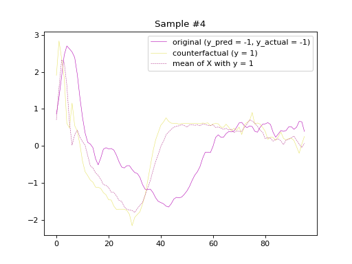
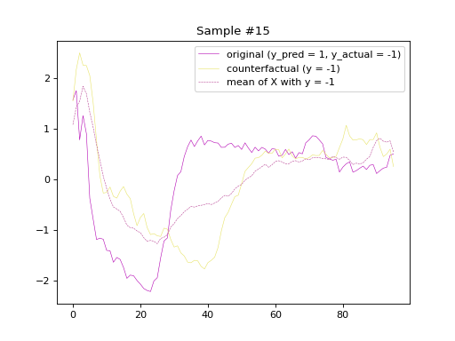
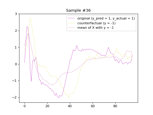
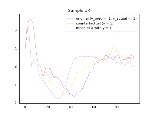
We now have three arrays: X_cf, y_pred, and cf_pred, which contain the counterfactual samples, the predicted labels of the original samples, and the predicted labels of the counterfactual samples, respectively. Subsequently, we will plot the original and counterfactual samples with indices 4 and 36, alongside the Euclidean average time series of the desired class.

Download plot source

Shapelet forest counterfactuals

One of the first methods for computing counterfactual explanations for time series was proposed by Karlsson et al. (2018) [2] and the proposed method make use of the random shapelet trees that are part of a random shapelet forest. In Wildboar, the random shapelet forest is implemented in the class ShapeletForestClassifier and we can construct counterfactuals for a shapelet forest using the class ShapeletForestCounterfactual.

Reusing the same dataset as for the k-nearest neighbors classifier, we can fit a shapelet forest classifier.

from wildboar.ensemble import ShapeletForestClassifier

rsf = ShapeletForestClassifier(
   n_estimators=100,
   metric="euclidean",
   max_depth=5,
   random_state=1,
)
rsf.fit(X_train, y_train)

ShapeletForestClassifier(max_depth=5, random_state=1)

In a Jupyter environment, please rerun this cell to show the HTML representation or trust the notebook.
On GitHub, the HTML representation is unable to render, please try loading this page with nbviewer.org.

The resulting estimator has an accuracy of 80.0%.

To compute counterfactuals, we use the class ShapeletForestCounterfactual in conjunction with the find_counterfactuals function defined previously. Counterfactuals are generated by traversing each predictive path within the decision trees that lead to the target outcome, and by modifying the most closely matching shapelets in the time series to ensure that the specified conditions are met.

from wildboar.explain.counterfactual import ShapeletForestCounterfactual
explainer = ShapeletForestCounterfactual(random_state=1)
X_cf, y_pred, cf_pred = find_counterfactuals(rsf, explainer, X_test)
X_cf

array([[ 0.64275557,  1.96522188,  2.90476179, ...,  0.09269015,
         0.12069088,  0.34982908],
       [ 0.5807386 ,  1.09711063,  1.74405634, ...,  0.28666866,
         0.32964692,  0.14763103],
       [ 0.5347352 ,  1.15122819,  2.66537309, ..., -0.31634668,
        -0.43290016, -0.38359833],
       ...,
       [ 0.29476759,  0.86093158,  2.41918778, ...,  0.16256033,
        -0.0061831 ,  0.56791544],
       [ 0.66077834,  0.7870391 ,  1.20106232, ...,  0.18811169,
         0.37941185,  0.32272574],
       [ 0.74926655,  0.33281894,  0.20372777, ...,  0.41850936,
        -1.25302505, -0.48742855]])

Download plot source

References

[1]

Karlsson, I., Rebane, J., Papapetrou, P. and Gionis, A., 2020. Locally and globally explainable time series tweaking. Knowledge and Information Systems, 62(5), pp.1671-1700.

[2]

Karlsson, I., Rebane, J., Papapetrou, P. and Gionis, A., 2018, November. Explainable time series tweaking via irreversible and reversible temporal transformations. In 2018 IEEE International Conference on Data Mining (ICDM) (pp. 207-216). IEEE.