Counterfactuals

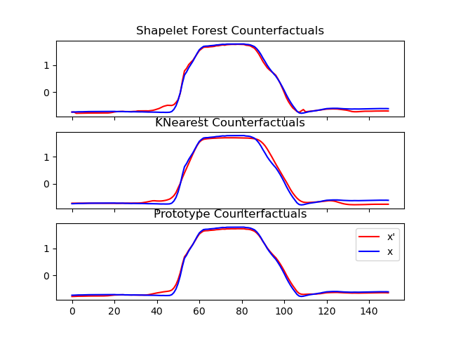
Comparison of counterfactual explanations

The following example show a few ways of computing counterfactual explanations.

import numpy as np
import matplotlib.pylab as plt
from sklearn.ensemble import RandomForestClassifier
from sklearn.model_selection import train_test_split
from sklearn.neighbors import KNeighborsClassifier

from wildboar.ensemble import ShapeletForestClassifier
from wildboar.datasets import load_dataset
from wildboar.explain.counterfactual import counterfactuals

random_state = 1234
x, y = load_dataset("GunPoint")

x_train, x_test, y_train, y_test = train_test_split(
    x, y, test_size=0.2, random_state=random_state
)

classifiers = [
    (
        "Shapelet Forest Counterfactuals",
        ShapeletForestClassifier(
            metric="euclidean", random_state=random_state, n_estimators=100
        ),
    ),
    ("KNearest Counterfactuals", KNeighborsClassifier(metric="euclidean")),
    ("Prototype Counterfactuals", RandomForestClassifier(random_state=random_state)),
]

fig, ax = plt.subplots(nrows=3, sharex=True)
label = np.unique(y_train)[0]
for i, (name, clf) in enumerate(classifiers):
    clf.fit(x_train, y_train)
    x_test_sample = x_test[y_test != label]
    if isinstance(clf, RandomForestClassifier):
        kwargs = {"background_x": x_train, "background_y": y_train}
    else:
        kwargs = {}

    x_counterfactual, valid = counterfactuals(
        clf, x_test_sample, label, random_state=random_state, **kwargs
    )
    ax[i].set_title(name + ("(invalid)" if not valid[0] else ""))
    ax[i].plot(x_counterfactual[0], c="red")
    ax[i].plot(x_test[0], c="blue")

ax[-1].legend(["x'", "x"])
plt.savefig("../fig/counterfactuals.png")