Annotate#
MatrixProfile#
The matrix profile is a data structure and accompanying algorithms that provide valuable insights into time series data. It was introduced by Yeh et al (2016), and is designed to solve various time series problems in a computationally efficient manner.
Recall that a time series is a sequence of data points typically measured at successive points in time, spaced at uniform time intervals. Examples include daily stock prices, monthly rainfall amounts, yearly temperatures, etc. In the context of time series, a subsequence is a contiguous portion of the time series. For example, if you have daily temperature readings for a year, a subsequence might be the temperatures from June 1 to June 30.
One of the primary applications of the matrix profile is motif discovery. A motif in time series analysis is a pattern (or subsequence) that occurs frequently. Identifying motifs can be crucial for understanding repetitive behaviors or trends in the data. The matrix profile can also help in detecting anomalies, which are subsequences that differ significantly from the rest of the time series. These can indicate errors, extraordinary events, or other significant deviations from the norm. Beyond motif discovery and anomaly detection, the matrix profile can be used for tasks such as time series forecasting, clustering, classification, and segmentation.
In summary, the matrix profile is a powerful tool for time series analysis that can help uncover patterns, detect anomalies, and perform various other analytical tasks on sequential data.
MatrixProfile data structure#
The matrix profile itself is a vector that stores the z-normalized Euclidean distance between each subsequence within a time series and its nearest, non-trivial match. A non-trivial match is the most similar subsequence that is not trivially similar (i.e., not overlapping significantly with the subsequence in question). The original algorithm to compute the matrix profile, STOMP (Scalable Time series Ordered-search Matrix Profile), and its subsequent improvements like STAMP (Scalable Time series Anytime Matrix Profile) and SCRIMP (Scalable Column-wise Recomputation of the Matrix Profile), allow for efficient computation of the matrix profile even for very large datasets.
The Matrix Profile Index (MPI) is a data structure that accompanies the Matrix Profile, which is a novel algorithmic technique used for time series data analysis. The Matrix Profile itself is a vector that stores the z-normalized Euclidean distance of each subsequence within a time series to its nearest neighbor. This information is extremely useful for various time series tasks such as anomaly detection, motif discovery (finding repeated patterns), and discord discovery (finding unusual patterns).
The Matrix Profile Index is a companion vector to the Matrix Profile and it stores the indices of the nearest neighbors. Each element of the Matrix Profile Index corresponds to an element in the Matrix Profile and indicates the location within the time series of the nearest neighbor for that subsequence.
Together, the Matrix Profile and Matrix Profile Index provide a powerful tool for understanding the structure and patterns within time series data. They enable efficient solutions to many time series problems and are particularly useful because they can be computed in a relatively efficient manner, often allowing for scalability to very large datasets.
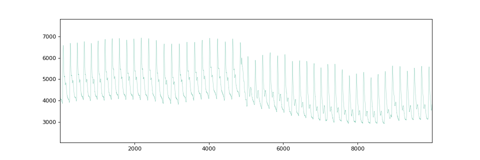
To exemplify the use of the matrix profile, we first load a time series and plot it:
import numpy as np
import matplotlib.pylab as plt

from wildboar.utils.plot import plot_time_domain

X = np.loadtxt(
    "https://drive.google.com/uc?export=download&id=1DYG3rwW_zpd-7lcgYeL0Y2nHtkr2Fi0O"
)
X = X[20000:30000]

fig, ax = plt.subplots(figsize=(12, 4))
plot_time_domain(X, ax=ax)
We can import matrix_profile to compute the matrix
profile for the time series:
from wildboar.distance import matrix_profile

mp, mpi = matrix_profile(X, window=200, return_index=True, kind="paired")
The matrix_profile-function returns the matrix profile (mp) and
optionally the matrix profile index if requested (if we set
return_index=True).
fig, ax = plt.subplots(nrows=2, figsize=(8, 4), sharex=True)
plot_time_domain(X, ax=ax[0])
plot_time_domain(mp, ax=ax[1])
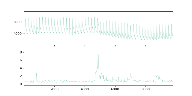
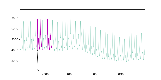
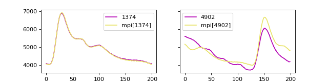
If we plot the matrix profile and the time series, we can observe that the
minimum MP value is at 1374 and the maximum value is at
4902. We can then use the MPI to discover that the MPI of
1374 is at mpi[mp.argmin()], that is at
2155.
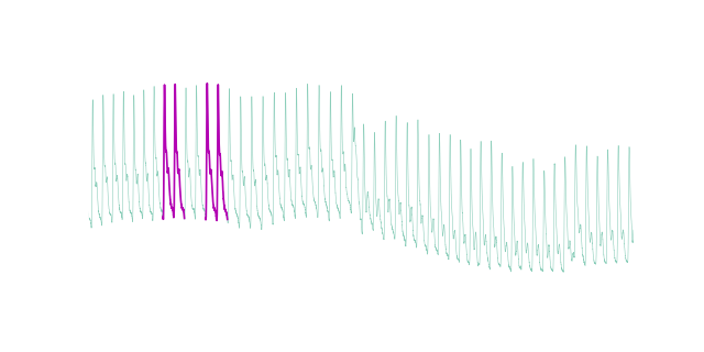
We can plot the sub-sequences to observe the (dis)similarity:
Motif discovery#
Motif discovery in time series refers to the process of identifying patterns or sub-sequences that recur within a longer time series data set. These motifs are significant because they often represent a behavior or feature that occurs repeatedly over time. The discovery of these motifs can provide insights into the underlying system that generated the time series, enabling better understanding, prediction, and anomaly detection. The process typically involves searching for subsequences that are similar to each other based on a predefined similarity threshold, which can be done using various algorithms such as brute force search, hashing, or more sophisticated methods like matrix profiles.
In Wildboar, we implement the approach described by Yeh (2016) [1]
in the function motifs. The function uses the matrix
profile identify the time series which has the closest neighbors and selects
those as motif candidates.
from wildboar.annotate import motifs

motif_indices = motifs(X, mp=mp, max_motifs=1, max_distance=0.5)
[array([1374, 2155, 1568, 2356])]
We can plot the motifs: