Tree-based estimators#

Shapelet-based decision trees#

For classification purposes, Wildboar provides two variants of shapelet trees. Both types of trees utilize random sampling of shapelets. The tree.ShapeletTreeClassifier selects shapelets in a random fashion, whereas the tree.ExtraShapeletTreeClassifier additionally samples the distance threshold at random. Correspondingly, both tree.ShapeletTreeRegressor and tree.ExtraShapeletTreeRegressor are implemented for regression tasks.

Since the trees are built using a (small) random sample of shapelets the predictive performance of a simple tree is poor. The model above has an accuracy of 77.3%.

We can increase the accuracy by increasing the size of the random sample:

The new estimator has an accuracy of 89.3%.

Interval-based decision trees#

Interval-based decision trees uses values computed for contiguous intervals. For example, we can construct a decision tree that uses the mean of intervals:

The classifier chooses the interval with the mean-value that optimizes the impurity criterion. The resulting estimator has an accuracy of 83.3%.

We can also build the tree either of the mean, variance or slope of the intervals:

The resulting estimator has an accuracy of 78.0%.

We can also use the catch22 features:

The resulting estimator has an accuracy of 94.7%.

Warning

If we compute more than one attribute value per interval, each node is split using a randomly drawn attribute value. The trees are more suitable in ensembles than as single trees.

One can also specify a list of callable functions that compute the attribute value for an interval:

The resulting estimator has an accuracy of 83.3%.

Warning

Wildboar trees are able to release the global interpreter lock unless a callable is passed. Using callable summarizers result in degraded performance.

Decision tree structure#

All decision tree estimators in Wildboar has an attribute tree_ which contains the low-level representation of the tree. The tree contains several parallel arrays that store the entire structure of the decision tree, for example the property tree_.max_depth records the maximal depth of the decision tree and tree_.node_count store the total number of (branch, leaf) nodes.

The arrays are indexed from [0, tree_.node_count) where 0 indicates the root node of the tree and the other indices refers to either a leaf or a branch node. We use the same array for both branches and leafs, meaning that some values are undefined for leafs or branches depending on its use. For example, the tree_.value records the values of leaf nodes, as such if the node is a branch the corresponding value is undefined. Similarly, the tree_.threshold array records the threshold used to partition the samples and is undefined if the node is a leaf-node.

The following arrays are available:

left: the id of the left node, e.g., left[0] corresponds to the left node after the root. The value is -1 if the node is a leaf.
right: the id of the right node, e.g., right[0] corresponds to the right node after the root. The value is -1 if the node is a leaf.
threshold: the threshold at a given node. The value is undefined for leaf nodes.
attribute: the attribute at a given node. The value is None for leaf nodes and a tuple (dim, attr) for branch nodes. The attr value depends on the decision tree.
value: the output value for the node id. The array has the shape (node_count, n_labels) where n_labels==1 for regression. The j:th column refers to the j:th class as present in the classes_ attribute. The value is undefined for branch nodes.
impurity: the impurity at the node.
n_node_samples: the number of samples reaching the node.
weighted_n_node_samples: the number of wheighted samples reaching the node. The same as n_node_samples unless sample_weight or class_weight is set.

We can compute various properties of the trees using these arrays. For example, we can obtain the decision path, that is the nodes a sample traverses or the terminal leaf reached by samples. Both methods are already provided by Wildboar as the methods decision_path and apply. First we construct a decision tree:

The decision tree has an accuracy of 95.3%.

Next, the following code sample shows the decision rules used to reach a prediction for a sample:

from wildboar.distance import pairwise_subsequence_distance

node_indicator = clf.decision_path(X_test)
leaf_id = clf.apply(X_test)
attribute = clf.tree_.attribute
threshold = clf.tree_.threshold
value = clf.tree_.value

sample_id = 100
# obtain ids of the nodes `sample_id` goes through, i.e., row `sample_id`
node_index = node_indicator.indices[
    node_indicator.indptr[sample_id] : node_indicator.indptr[sample_id + 1]
]

print("Rules used to predict sample {id}:\n".format(id=sample_id))
for node_id in node_index:
    # continue to the next node if it is a leaf node
    if leaf_id[sample_id] == node_id:
        continue

    # check if value of the split feature for sample 0 is below threshold
    (dim, (_, shapelet)) = attribute[node_id]
    dist = pairwise_subsequence_distance(
        shapelet, X_test[sample_id], metric="scaled_euclidean"
    )
    if dist <= threshold[node_id]:
        threshold_sign = "<="
    else:
        threshold_sign = ">"

    print(
        f"decision node {node_id} : (D(X_test[{sample_id}], S[{node_id}]) = {dist}) "
        f"{threshold_sign} {threshold[node_id]})"
    )

Rules used to predict sample 100:

decision node 0 : (D(X_test[100], S[0]) = 1.1344171278001063) > 0.9142979223080065)
decision node 4 : (D(X_test[100], S[4]) = 1.0061231459189364) > 0.8250243865539288)

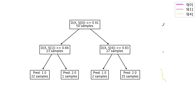
Plotting#

We can plot shapelet-based decision trees using the plot_tree function.

from wildboar.tree import plot_tree

plot_tree(clf)

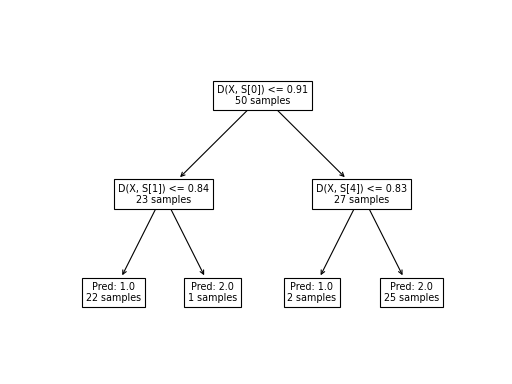
In the tree decision tree, we observe three branching nodes and four terminal nodes. Each node displays the count of samples that have reached it. For example, the initial branching node is reached by the entire training set (50 samples), while the leftmost terminal node is reached by 22 samples. The branching nodes define the decision criteria that determine the path to follow: the left path is taken if the distance between the sample and the shapelet is less than the threshold, and the right path is taken if the distance exceeds the threshold. This criterion is represented in the node by the inequality D[X, S[0]] <= 0.91, which signifies that if the distance between the sample and the first shapelet is less than 0.91, the left path is chosen (conversely, the right path is chosen if the distance is greater). Upon reaching a terminal node, the prediction, denoted by Pred: y, is assigned to the sample.

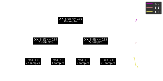
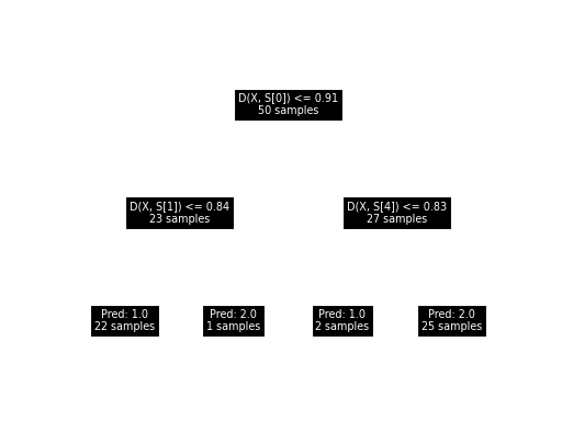
We can also visualize the samples together with the tree:

Download source