Segmentation

Time series segmentation is a process used to divide a time series, which is a sequence of data points indexed in time order, into multiple segments or sections that are more homogeneous or have distinct characteristics. The goal of segmentation is to simplify the analysis by breaking down a complex time series into pieces that are easier to understand and analyze. Each segment can be thought of as representing a different behavior or regime within the data.

When using the matrix profile for time series segmentation, the goal is to identify points in the time series where the properties of the data change significantly, which are often referred to as change points. The matrix profile helps in this task by highlighting areas where the distance to the nearest neighbor suddenly changes. These changes can indicate potential boundaries between segments.

By analyzing the matrix profile, one can detect these change points more efficiently than with many traditional methods, which often require more computation and may not be as effective at handling large or complex time series data. Once the change points are identified, the time series can be segmented accordingly, allowing for further analysis on each individual segment, such as trend analysis, anomaly detection, or forecasting, with each segment being treated as a separate entity with its own characteristics.

In Wildboar, we can segment a time series using the matrix profile with the FlussSegmenter class.

import numpy as np
import matplotlib.pylab as plt

x = np.loadtxt(
    "https://drive.google.com/uc?export=download&id=1DYG3rwW_zpd-7lcgYeL0Y2nHtkr2Fi0O"
)
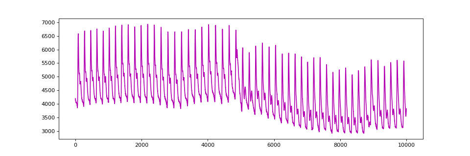
X = x[20000:30000].reshape(1, -1)

Download source

Next, we import the segmenter and fit it to the data, specifying the number of segments, n_segments, as two, and setting the boundary parameter to 1, which corresponds to the full window size. We utilize a window size of 200. It is important to note that the window size is a parameter that requires considerable tuning and may necessitate domain expertise to properly adjust.

A segmenter exposes two primary functions: predict and transform. When provided with a previously unseen sample, both methods use the closest sample to assign the segments. However, typically the same data used to fit the segmenter is also used to predict the segmentation. The predict function returns a sparse boolean matrix with the indices of the segments set to 1; whereas the transform function returns an array with each time step annotated with the segment to which it belongs.

s.predict(X).nonzero()

(array([0, 0]), array([4902, 5265]))

Thus, the first segment starts at 4902 and the second segment starts at 5265. Similarly, we can use the predict-function to cluster the points:

Xt = s.transform(X)

Since the transform returns an array with the cluster labels in ascending order, we can count the number of labels to get the start and end of each segment:

unique, start, count = np.unique(
    Xt[0], return_counts=True, return_index=True, equal_nan=True
)
segments = [(start, start + count) for start, count in zip(start, count)]

[(np.int64(0), np.int64(4902)), (np.int64(4902), np.int64(5265)), (np.int64(5265), np.int64(10000))]

Next we can overlay the time series with the regions in the time series (n_segments + 1 regions).

Download source