Dynamic time warping

In this example, we use dynamic time warping (DTW) and Weighted DTW.

import matplotlib.pylab as plt
from matplotlib.collections import LineCollection
from wildboar.datasets import load_dataset
from wildboar.distance.dtw import (
    dtw_alignment,
    wdtw_alignment,
    dtw_mapping,
    dtw_distance,

)

First, we load a dataset.

data, _ = load_dataset("Wafer")
x = data[0]
y = data[1]

Next, we define a function that we use to plot the alignment between two time series under DTW.

def plot_alignment(x, y, idx):
    fig, ax = plt.subplots(figsize=(10, 5))
    ax.plot(x)
    ax.plot(y)

    lines = [[(a, x[a]), (b, y[b])] for a, b in zip(*idx)]
    collection = LineCollection(lines, color="gray", linewidth=0.5)
    ax.add_collection(collection)

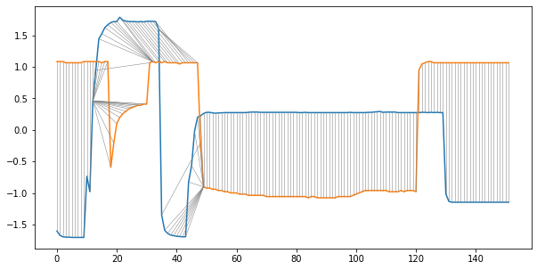
Dynamic Time Warping

In the first exampe, we use traditional dynamic time warping and a band of size 7.

plot_alignment(x, y, dtw_mapping(alignment=dtw_alignment(x, y, r=0.05)).nonzero())

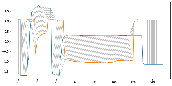
Weighted Dynamic Time Warping

In the second example, we plot the alignment path under weighted DTW with the penelty parameter set to 0.5.

plot_alignment(x, y, dtw_mapping(alignment=wdtw_alignment(x, y, g=0.05)).nonzero())