Matrix profile

The matrix profile is a data structure that annotates a time series with the distance of the closest matching subsequence at the i:th index. In these examples, we explore the use of the matrix profile and motif and regime change detection as implemented in terms of it.

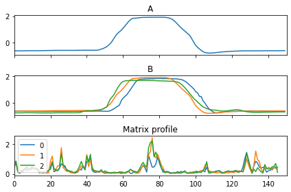
Similarity AB-join

In the first example, we join every subsequence in the second sample with the first three samples.

import numpy as np
import matplotlib.pylab as plt

from wildboar.datasets import load_dataset
from wildboar.distance import matrix_profile, subsequence_match

First, we load a dataset.

x, y = load_dataset("GunPoint")

Second, we compute the matrix profile similarity join between the first three samples and the second sample.

mp = matrix_profile(x[0:3], x[1], window=5, exclude=0.2)

Finally, we plot the samples and the matrix profile

fig, ax = plt.subplots(nrows=3, sharex=True)
ax[0].plot(x[1])
for i in range(mp.shape[0]):
    ax[1].plot(x[i], label=str(i))
    ax[2].plot(mp[i], label=str(i))

ax[0].set_title("A")
ax[1].set_title("B")
ax[2].set_title("Matrix profile")
ax[0].set_xlim(0, x.shape[-1])
ax[1].set_xlim(0, x.shape[-1])
ax[2].set_xlim(0, x.shape[-1])
plt.legend()
plt.tight_layout()

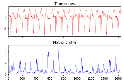
Similarity self-join

In the second example, we self-join every subsequence with its closest position. First, we load a dataset and concatenate the first 20 samples.

x, y = load_dataset("TwoLeadECG")
x = x[:20].reshape(-1)

Second, we compute the matrix profile self-join.

mp = matrix_profile(x.reshape(-1), window=20, exclude=0.2)

Finally, we plot the time series and matrix profile

fig, ax = plt.subplots(nrows=2, sharex=True)
ax[0].plot(x, color="red", lw=0.5)
ax[1].plot(mp, color="blue", lw=0.5)
ax[0].set_title("Time series")
ax[1].set_title("Matrix profile")
ax[0].set_xlim(0, x.shape[-1])
ax[1].set_xlim(0, x.shape[-1])
plt.tight_layout()

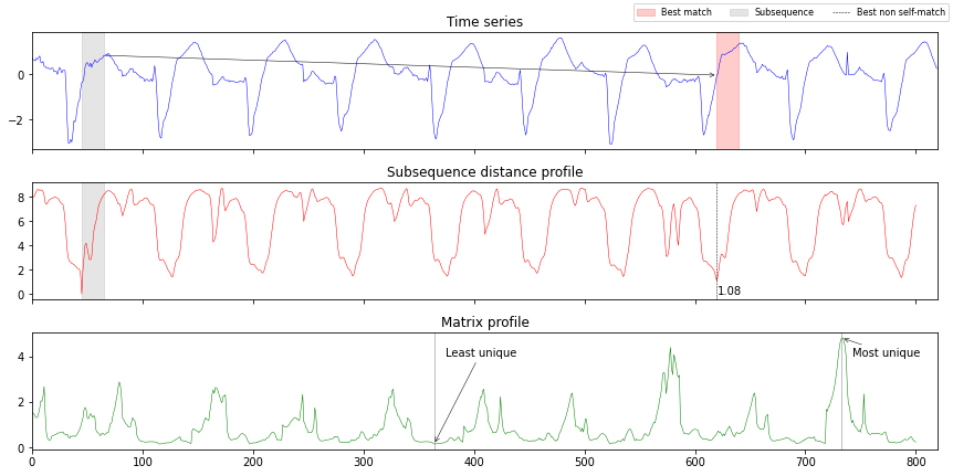
Matrix profile and subsequence distance

In the third example, we

First, we load a dataset concatenating the first 10 samples and extracting a subsequence of 20 timesteps, starting at index 45.

x, y = load_dataset("TwoLeadECG", preprocess="normalize")
x = x[0:10].reshape(-1)
subseq = x[45:65]

Second, we compute the distance to all matching same-length subsequences.

idx, dist = subsequence_match(
    subseq.reshape(1, -1),
    x.reshape(1, -1),
    return_distance=True,
    threshold=np.inf,
    metric="scaled_euclidean"
)
do = np.argsort(dist)

Next, we compute the self-join matrix profile.

mp, mpi = matrix_profile(x, window=20, return_index=True)
lu = np.argmin(mp)
mu = np.argmax(mp)

fig, (ax1, ax2, ax3) = plt.subplots(nrows=3, figsize=(12, 6), sharex=True)

ax1.set_title("Time series")
ax1.plot(x, color="blue", lw=0.5)
ax1.set_xlim(0, x.size)
ax1.axvspan(45, 65, 0, 1, color="gray", alpha=0.2)
ax1.annotate(text="", xy=(65, x[65]), xytext=(mpi[45], x[mpi[45]]), arrowprops=dict(arrowstyle='<-', lw=0.5))
ax1.axvspan(mpi[45], mpi[45]+20, 0, 1, color="red", alpha=0.2, label="Best match")

ax2.set_title("Subsequence distance profile")
ax2.plot(idx, dist, color="red", lw=0.5)
ax2.axvspan(45, 65, 0, 1, color="gray", alpha=0.2, label="Subsequence")
ax2.annotate(text="%.2f" % dist[do[1]], xy=(do[1], x[do[1]]))
ax2.axvline(do[1], 0, 1, color="black", lw=0.5, ls="--", label="Best non self-match")

ax3.set_title("Matrix profile")
ax3.plot(mp, color="green", lw=0.5)
ax3.axvline(lu, 0, 1, color="gray", lw=0.5)
ax3.annotate(text="Least unique", xy=(lu, mp[lu]), xytext=(lu + 10, 4), arrowprops=dict(arrowstyle='->', lw=0.5))
ax3.axvline(mu, 0, 1, color="gray", lw=0.5)
ax3.annotate(text="Most unique", xy=(mu, mp[mu]), xytext=(mu + 10, 4), arrowprops=dict(arrowstyle='->', lw=0.5))
fig.tight_layout()
fig.legend(ncol=4, fontsize=8)

<matplotlib.legend.Legend at 0x7faf80dcdf10>