Counterfactual explanations

wildboar can explain predictions of nearest neighbors classifiers and shapelet forest classifiers using counterfactual samples. In this scenario, counterfactuals are samples that are transformed such that the labeling of the sample changes. For instance, we might want to explain what changes are required to transforms a sample labeled as abnormal to normal. In this scenario, the normal sample would be the counterfactual sample.

In wildboar, counterfactual explainers are in the module wildboar.explain.counterfactual. The easiest way to generate counterfactuals is to use the function counterfactuals:

from wildboar.explain.counterfactual import counterfactuals

Currently, the classifiers that supports counterfactual explanations are ShapeletForestClassifier and KNearestNeighborsClassifier from wildboar and scikit-learn respectively. Model agnostic counterfactual explanations can be provided for any other estimators.

To have more control over the generation of counterfactual samples, the classes KNeighborsCounterfactual and ShapeletForestCounterfactuals can be used. They implement the interface of BaseCounterfactuals which exposes two methods fit(estimator) and transform(x, y), where the former fits a counterfactual explainer to an estimator and the latter transform the i:th sample of x to a sample labeled as the i:th label in y.

import numpy as np
import matplotlib.pylab as plt
from wildboar.datasets import load_dataset
from wildboar.explain.counterfactual import KNeighborsCounterfactual
from sklearn.neighbors import KNeighborsClassifier

That is, given

x_train, x_test, y_train, y_test = load_dataset("GunPoint", merge_train_test=False)
clf = KNeighborsClassifier(n_neighbors=5, metric="euclidean")
clf.fit(x_train, y_train)

KNeighborsClassifier(metric='euclidean')

In a Jupyter environment, please rerun this cell to show the HTML representation or trust the notebook.
On GitHub, the HTML representation is unable to render, please try loading this page with nbviewer.org.

c = KNeighborsCounterfactual(random_state=123)
c.fit(clf)
x_test = x_test[y_test != 1]
y_cf = np.ones(x_test.shape[0])
counterfactual = c.explain(x_test, y_cf)

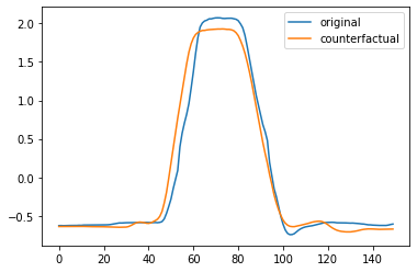
plt.plot(x_test[0])
plt.plot(counterfactual[0])
plt.legend(["original", "counterfactual"])

<matplotlib.legend.Legend at 0x7faf58698f40>

Warning

KNeighborsCounterfactuals only supports KNeighborsClassifier fit with the Euclidean distance.

Evaluating counterfactuals

Good counterfactuals should be plausible (i.e., inside the distribution), valid (i.e., of the desired label as measured by the classifier), close to the original (i.e., have low proximity) and sparse (i.e., have as few changes introduced as possible).

from wildboar.metrics import (
    proximity_score,
    relative_proximity_score,
    validity_score,
    plausability_score,
    compactness_score,
)

proximity_score(x_test, counterfactual)

4.459784399792326

validity_score(y_cf, clf.predict(counterfactual))

0.8918918918918919

plausability_score(x_train, counterfactual)

0.6891891891891891

compactness_score(x_test, counterfactual)

9.009009009009009e-05

relative_proximity_score(x_train[y_train == 1], x_test, counterfactual)

1.0809175254653052

Example

In the following example, we explain the a nearest neighbors classifier and a shapelet forest classifier for the datasets TwoLeadECG and explaining samples classified as 2.0 if they instead where classified as 1.0 (in the legend denoted as abnormal and normal respectively).

import numpy as np
from sklearn.model_selection import train_test_split
from wildboar.ensemble import ShapeletForestClassifier
from wildboar.explain.counterfactual import counterfactuals

x, y = load_dataset("TwoLeadECG")
x_train, x_test, y_train, y_test = train_test_split(
    x, y, test_size=0.1, random_state=123
)

estimator = ShapeletForestClassifier(random_state=123, n_shapelets=10, n_jobs=-1, metric="euclidean")
estimator.fit(x_train, y_train)
x_test = x_test[y_test == 2.0]
x_counterfactuals, valid, proximity = counterfactuals(
    estimator,
    x_test,
    1.0,
    proximity="euclidean",
    random_state=123,
)

x_test = x_test[valid]
x_counterfactuals = x_counterfactuals[valid]
i = np.argsort(proximity[valid])[:2]
x_counterfactuals = x_counterfactuals[i, :]
x_test = x_test[i, :]

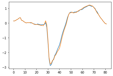
Plotting the counterfactual with the lowest score, yields the following figure.

plt.plot(x_test[0])
plt.plot(x_counterfactuals[0])

[<matplotlib.lines.Line2D at 0x7faf491392e0>]

plausability_score(x_train, x_counterfactuals)

1.0

relative_proximity_score(x_train[y_train == 1], x_test, x_counterfactuals)

0.5663516974015599

proximity_score(x_test, x_counterfactuals)

0.6691132421072039