Comparing counterfactals

In these examples, we will explore counterfactual explanations of time series classifiers. The goal of counterfactual explanations is to highlight the changes required to transform a time series predicted as a particular class to a time series as predicted as another class, i.e., showing the changes required to change the predictors outcome.

import matplotlib.pylab as plt
import numpy as np
from sklearn.ensemble import RandomForestClassifier
from sklearn.neighbors import KNeighborsClassifier
from sklearn.model_selection import train_test_split

from wildboar.datasets import load_dataset
from wildboar.ensemble import ShapeletForestClassifier
from wildboar.explain.counterfactual import (
    counterfactuals,
    ShapeletForestCounterfactual,
    KNeighborsCounterfactual,
    PrototypeCounterfactual,
)

random_state = 1234

As usual, the first step is to load a dataset and split it into training and testing partitions.

x, y = load_dataset("TwoLeadECG")

x_train, x_test, y_train, y_test = train_test_split(
    x, y, test_size=0.2, random_state=random_state
)
label = np.unique(y_train)[0]
x_test_sample = x_test[y_test != label][:2]

Next, we will explore counterfactual explanations for three classifiers

• RandomShapeletForest

• KNearestNeighborsClassifier

• and, the traditional, RandomForestClassifier

We explore couterfactuals computed for the random shapelet forest as computed by the local counterfactual algorithm. Note that the metric="euclidean" is required for this counterfactual method.

clf = ShapeletForestClassifier(
    metric="euclidean", random_state=random_state, n_estimators=100
)
clf.fit(x_train, y_train)

ShapeletForestClassifier(random_state=1234)

In a Jupyter environment, please rerun this cell to show the HTML representation or trust the notebook.
On GitHub, the HTML representation is unable to render, please try loading this page with nbviewer.org.

Second, we fit the counterfactual explanation to the given estimator.

explain = ShapeletForestCounterfactual(random_state=random_state)
explain.fit(clf)

ShapeletForestCounterfactual(random_state=1234)

In a Jupyter environment, please rerun this cell to show the HTML representation or trust the notebook.
On GitHub, the HTML representation is unable to render, please try loading this page with nbviewer.org.

When predicting, the shapelet forest accurately predict the samples as label 2.

clf.predict(x_test_sample)

array([2., 2.], dtype=float32)

In an effort to explain those predictions, we exploit the counterfactual engine to transform the samples to the desired label (1 in the example). Note that the transform-function, expects one or more samples and one or more desired outcomes. Below, we want all samples to be explained as 1, so we simply broadcast the scalar to an array with as many rows as x_test_sample.

x_counterfactual = explain.transform(
    x_test_sample, np.broadcast_to(label, (x_test_sample.shape[0],))
)

Next, we ensure that the counterfactuals are indeed predicted as the desired label by the classifier we try to explain.

clf.predict(x_counterfactual)

array([1., 1.], dtype=float32)

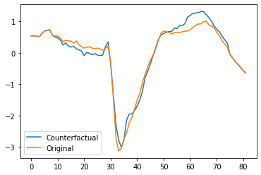
Finally, we plot the first counterfactual and original time series and find that there are two main regions which we need to change for the prediction to change.

plt.plot(x_counterfactual[0])
plt.plot(x_test_sample[0])
plt.legend(["Counterfactual", "Original"])

<matplotlib.legend.Legend at 0x7fd098f54280>

Since the counterfactual explanation interface is inconvenient, wildboar has a helper function counterfactuals which can be used to compute countefactuals for a given estimator.

x_counterfactual, valid, score = counterfactuals(
    clf,
    x_test_sample,
    label,
    scoring="euclidean",
    valid_scoring=True,
    random_state=random_state,
)

We can explore which counterfactuals are valid (i.e., those counterfactuals for which the classifier predicts the desired label).

valid

array([ True,  True])

And, we can also explore the score of the counterfactuals. Here, the scoure is the euclidean distance between the original and counterfactual time series.

score

array([1.6957227 , 1.03749523])

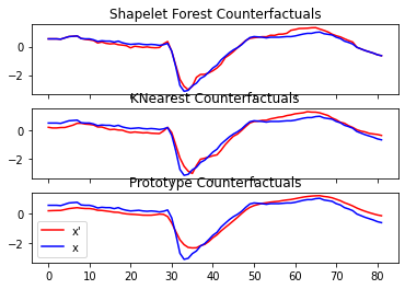
Finally, we can compare the counterfactuals of different methods and plot the output.

classifiers = [
    (
        "Shapelet Forest Counterfactuals",
        ShapeletForestClassifier(
            metric="euclidean", random_state=random_state, n_estimators=100, n_jobs=-1
        ),
    ),
    ("KNearest Counterfactuals", KNeighborsClassifier(metric="euclidean")),
    ("Prototype Counterfactuals", RandomForestClassifier(random_state=random_state)),
]

fig, ax = plt.subplots(nrows=3, sharex=True)
label = np.unique(y_train)[0]
for i, (name, clf) in enumerate(classifiers):
    clf.fit(x_train, y_train)
    x_test_sample = x_test[y_test != label][:2]
    if isinstance(clf, RandomForestClassifier):
        kwargs = {"train_x": x_train, "train_y": y_train}
    else:
        kwargs = {}

    x_counterfactual, valid = counterfactuals(
        clf, x_test_sample, label, random_state=random_state, method_args=kwargs
    )
    ax[i].set_title(name + ("(invalid)" if not valid[0] else ""))
    ax[i].plot(x_counterfactual[0], c="red")
    ax[i].plot(x_test[0], c="blue")

ax[-1].legend(["x'", "x"])

/Users/isak/Projects/wildboar/src/wildboar/explain/counterfactual/__init__.py:209: UserWarning: no specific counterfactual explanation method is available for the given estimator. Using a model agnostic estimator.
  warnings.warn(

<matplotlib.legend.Legend at 0x7fd0e93929d0>